Data Cleaning – the secret ingredient to the success of any Data Science Project

In the last few blogs, we saw how to summarise and analyse the data using statistical methods and visualisations. But the raw data need to be processed to convert it into a usable shape. Data Preparation is the most important and foremost part of Data Science. It involves data pre-processing and data wrangling. Raw data is collected from various sources and usually unsuitable for analysis. For example, there might be many entries for a shopper leading to duplicity, or there might a typo in noting down the email id of a customer, or some of the questions might have been left blank by a surveyor. With an uncleaned dataset, no matter what type of algorithm you try, you will never get accurate results. That is why data scientists spend a considerable amount of time on data cleaning. Better data beats fancier algorithms. Though, the steps and techniques for data cleaning will vary for each dataset. But the following steps could be used as a standard approach for any dataset type:

1. Identifying relevant data and removing irrelevant data
2. Fix Irregular cardinality and structural errors
3. Outliers
4. Missing data treatment

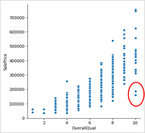
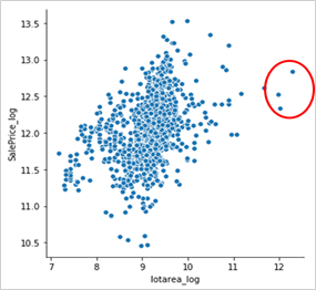
As discussed in the blog, running a basic descriptive statistics test provides an initial sense check of data in terms of missing values, variation in a feature, cardinality of features. Figure 1: Summary Statistics   Figure 2: Check for Null Values   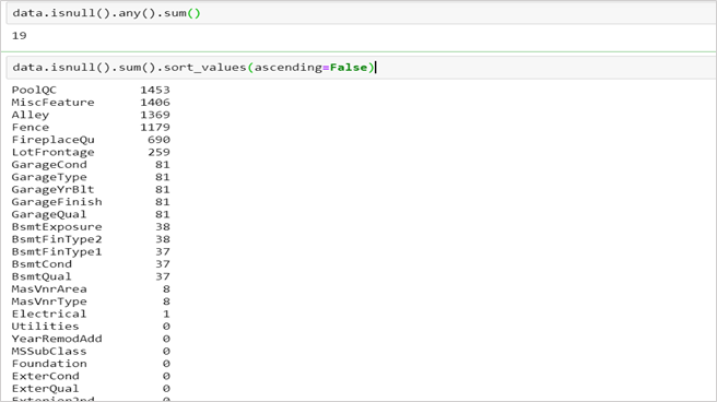Figure 3: Outliers highlighted in red  

Identifying relevant data and removing irrelevant data

Mainly two checks should be carried out for identifying irrelevant data: 1. Duplicate entries Data is usually collected from many sources and joined together to form one dataset. This might lead to the duplicity of observations. This might not be problematic if observations (small in number) are repeated a few times but could lead to erroneous behaviour if observation(s) are repeated far too many times. Hence, it is better to drop duplicate observations to have a cleaner dataset. 2. Irrelevant observations The dataset would contain observations which might not be useful for your specific task. For example, if you were analysing the shopping behaviour of women only, you would not require observations for men in your dataset — row-wise. Similarly, your data might have a column for id or names of employees which would not be very helpful in making predictions and could be dropped — column-wise.  

Fix Irregular cardinality and structural errors

1. Drop the columns which have a cardinality of 1 (for categorical features), or zero or very low variance (for continuous features). Such features do not provide much information and are not useful for building predictive models.
2. Categorical columns could have a high number of classes due to typos or inconsistent capitalization. For example, the gender column might have many classes like male, female, m, f, M, and F, these represent only two levels — Male and Female. Such classes should be mapped to proper levels and the rest of the levels should be dropped. Bar plots could be used to highlight such issues.
3. Ensure that the data is represented by the correct data type i.e. numbers are stored as int/float, date as a date object.

There could be many issues like whitespaces in the feature values, data in a feature could have mixed data types like a numerical column might have some numbers as numerals and some as strings or objects. Fixing such errors would result in a cleaner and easy to interpret and use dataset.  

Outliers

In the previous blog, we discussed ways to identify outliers. To summarise, data points could be treated as if the data points lie:

1. above Q3 + 1.5*IQR or below Q1–1.5*IQR, if the data follows a non-Gaussian distribution
2. 2 or 3 standard deviations away from the feature mean (z-score), if the data follows a Gaussian distribution
3. Visualise univariate variables by plotting Box plots, histograms or scatterplot (as shown in figure 3)

These methods are good for initial analysis of univariate or bivariate (scatterplot) variables but do not hold much value for multivariate data or data with high dimensions. For such cases, advanced methods like clustering, PCA, LOF (Local Outlier Factor) & HiCS: High Contrast Subspaces for Density-Based Outlier Ranking should be leveraged.  

Ways to deal with Outliers

1. To retain or to trim We should not drop any observations without careful consideration, as such information can be valuable to understand the unusual behaviour or anomalies in the data unless we are sure that the outlier may be due to measurement error or if the presence of outliers influences the fit of a model.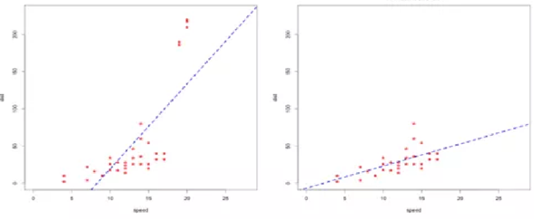 Figure 4: With Outliers (left pic), the regression line seems to be influenced by the extreme points in the top. Without Outliers (right pic). the regression line better fits the data after dropping the extreme points.  

2. Winsorising or Clamp Transformation: Winsorising replaces the outliers with the nearest nonsuspect data. This is also called clamp transformation as we clamp all values above an upper threshold and below a lower threshold to these threshold values, thus capping the values of outliers:

where fi is a specific value of feature f, and lower and upper are the lower and upper thresholds., given by either the IQR method or z-score discussed above.

It is recommended to apply the clamp transformation in cases where it is suspected that a model is performing poorly due to the presence of outliers. The better way to evaluate the impact of winsorising is by comparing the performance of different models trained on datasets where the transformation has been applied and where it has not.

 

3. Use algorithms robust to outliers

Tree-based algorithms and boosting methods are insensitive to outliers due to the intrinsic nature of the recursive binary splitting approach used to partition the feature space. These algorithms are the best bet when there are outliers in the input features. If there are outliers in the target variable, tree-based algorithms are good but care must be taken to choose the loss function. Reason being that if we use the mean squared error function, then the difference is squared and would highly influence the next tree since boosting attempts to fit the (gradient of the) loss. However, there are more robust error functions that can be used for boosted tree methods like Huber Loss and Mean Absolute Deviation loss.   Data Cleaning and Descriptive Statistics and EDA are a very important part of data science life cycle. Understanding the data is crucial to get high-level insights about the population behaviour and it also helps you decide which transformations to apply, if required and which algorithms would give best results for your specific business problem. We will talk about how to treat missing values in the next blog.     References: https://www.r-bloggers.com/outlier-detection-and-treatment-with-r/     Share this on


Follow us on